Fundamentals of Machine learning
Machine learning is an ever-changing and evolving field of study. But, understanding the latest and the state-of-the-art techniques require a strong knowledge of the foundations of Machine learning. I have started this series as a means to improve my knowledge and help someone who stumbles upon my blog. The posts are explanations for the slides from the Machine learning lectures at University of Liege.
Statistical learning
Statistical learning are the different methods for understanding data. They can be supervised or unsupervised depending on the situation.
Supervised learning
Supervised learning is a means of statistical learning where a model learns from a set of labeled data, with features representing different aspects of our data to model on and one or more targets to learn. The features depend on the problem, such as a tabular data containing details about the wind speed in different locations, an image represented as an array of its pixels, a raw audio and so on. The targets, too, vary depending on the problem, for example in a classification problem the target might represent the category each example belongs to, in a regression problem, it might represent a real value and in reinforcement learning it might represent the value of our policy.
Let \(X\) represent our features and \(Y\) represent our targets. Generally, we do not have any prior information about input probability distribution. Thus, the probability distribution is unknown to us. We also assume that the input is i.i.d (Independent and identically distributed). Let \(P(X, Y)\) be the unknown joint probability distribution of the input dataset.
If \(i\) indicates the i’th example from the finite input dataset with \(N\) examples, then a single instance of the dataset is
\[(x_i, y_i) \sim P(X, Y)\]where, \(x_i \in \mathcal X\), \(y_i \in \mathcal Y\), and \(i=1, ..., N\).
In most cases, the pair \((x_i, y_i)\) consists of a p-dimensional vector representing the features or descriptors and a scalar value representing a class, category or a real value.
Supervised learning problems are usually concerned with two inference problems:
-
Classification: Classification problems deal with classifying the input into a fixed set of categories. An example is classifying a random set of dogs and cat images to their respective classes. The ImageNet challenge is a famous challenge of image classification which is almost single handedly responsible for starting the revolution in Computer Vision.
In this problem, given a feature vector, and a target as a scalar or an one-hot encoded vector representing the corresponding class from the set of cartesian product of \(X\) and \(Y\), we predict the class with the highest probability given the input data. Mathematically,
Given, \((x_i, y_i) \in \mathcal X\times \mathcal Y = \mathbb R^{p} \times \Delta^{c},\) for \(i = 1, ..., N\), we want to estimate for any new \(x\),
\[\mathop{argmax}_{y} P(Y=y \mid X = x)\] -
Regression: Regression problems deal with predicting a value for the given input. This is prevalent in areas related to finance. An example is stock prediction in which a set of features is used to predict the price of a stock.
In this problem, given a pair of input data consisting of a set of features and the corresponding value, we predict the expected value. Mathematically,
Given \((x_i, y_i) \in \mathcal X \times \mathcal Y = \mathbb R^{p} \times \mathbb R\), for \(i=1, ..., N\), we want to estimate for any new \(x\),
\[\mathbb E[Y \mid X=x]\]
Empirical risk minimization
Machine learning models learn basically by minimizing a defined function. This function is called a loss function. If a model is improving, then its loss will steadily decrease to a stable value. The figure below shows a convex loss function, which is a bowl shaped function.
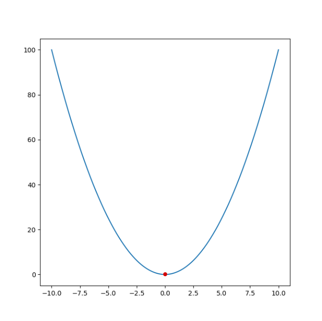
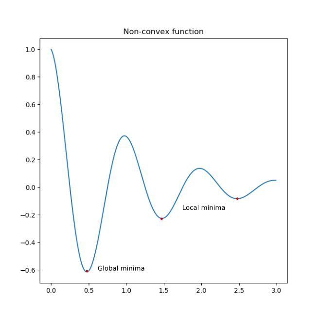
In a function, the lowest value possible is the global minimum (shown as a red point above). The loss function showed above has a single minimum which is the global minimum. As the model loss converges to zero, it is said to have reached a global minimum and is theoritically the optim4um value a model can reach. Unfortunately, not all functions are convex and modern machine learning architectures are riddled with complex loss function with multiple local minima and saddle points. A local minima is a value which is smallest in its vicinity but might not be the lowest point. A saddle point is a point which has the same value as its surrounding which can impede the training by getting stucked. Often times, a local optimum is good enough for most tasks.
Let us consider a function \(f : \mathcal X \to \mathcal Y\) (a function, f mapping from X, the features to Y, the targets) produced by some learning algorithm. We can evaluate this function with a loss function as,
\[\mathcal l: \mathcal Y \times \mathcal Y \to \mathbb R\]such that \(\mathcal l (y, f(x)) \ge 0\) measures how close the prediction \(f(x)\) from \(y\) is. The loss function takes two vectors: the ground truth (\(Y\)) and the predicted vector (say \(\hat Y\)) of the same dimensions and generates a single real number, the loss.
For a classification task, the loss function determines how far the predicted class is from the true class.
\[\mathcal l(y, f(x)) = 1_{y \ne f(x)}\]The function shows that it predicts 1 for a wrong class prediction i.e. when \(y \ne f(x)\).
For a regression problem, the loss function can be defined as:
\[\mathcal l(y, f(x)) = (y - f(x))^{2}\]The mean of this loss over all examples in the dataset gives us the Mean Squared Error (M.S.E) loss function. It determines how our predictions vary from the real value.
Let \(\mathcal F\) denote the hypothesis space. The hypothesis space is the set of all possibe functions \(\mathcal f\) produced by the chosen algorithms. It includes every possible function that can be generated from the chosen algorithm some of which might generalize very well to the chosen task while others might be sub-optimal.
We are looking for a function \(\mathcal f \in \mathcal F\) with a small expected empirical risk. This is also known as generalization error because a model generally performs better with a lower generalization error. Generally, we are interested in the model error in the test set of our data (which is often thought of as representative of real world data).
If \(R(f)\) denote the risk for function \(\mathcal f\) then,
\[R(f) = \mathbb E_{(\mathbf x , y) \sim P(X, Y)} [\mathcal l(y, f(\mathbf x))]\]It tells us that the expected risk, \(\mathcal R(f)\) is the average risk over all the examples in the dataset. Simply, if there are m examples in the dataset, the expected risk or average loss can be determined as,
\[R(f) = \frac{1}{m} \sum_{i=1}^{m} \mathcal l(y, f(x))\]Thus, we can say that for a given data generating distribution \(P(X, Y)\) and for a given hypothesis space \(\mathcal F\), the optimal model is
\[\mathcal f_{\star} = \mathop{argmin}_{\mathcal f \in \mathcal F} R(f)\]we are selecting function \(f\) with minimum expected risk. Since, this is the one with the minimum generalization error, it is what we wish to obtain but it is rarely possible in practice.
In practice, we do not know the input data distribution \(P(X, Y)\) and thus, the expected risk cannot be evaluated directly and the optimal model cannot be determined.
However, with the assumption that the data we obtained is i.i.d (independent and identically distributed), we can estimate the empirical risk. Let \(\mathbf d=\{(\mathbf x_{i}, y_i) \mid i=1, ..., N\}\) be the training data, then an estimation of the empirical risk can be determined as:
\[\hat{R} (\mathcal f, \mathbf d ) = \frac{1}{N} \sum_{(\mathbf x_{i}, y_i) \in \mathbf d } \mathcal l(y_i, f(\mathbf x_{i}))\] \[\color{red}{Add\ Explanation: Unbiased\ estimator}\]This is an unbiased estimation of the generalization error and with enough data we can find a good enough approximation of \(\mathcal f_{\star}\). This results in the empirical risk minimization principle.
\[\mathcal f_{\star}^{d} = \mathop{argmin}_{\mathcal{f \in F}} \hat{R}(f, \mathbf d)\]This says that the best estimation of the function \(\mathcal f\) is the one which has the minimum empirical risk.
\[\color{red}{Add\ Explanation: Regularity\ assumption}\]In practice, most machine learning algorithms implement empirical risk minimization. Under regularity assumption, empirical risk minimizers converge:
\[\lim \limits_{N \to \infty} \mathcal f_{\star}^{d} = \mathcal f_{*}\]Linear Regression
Linear Regression, as the name suggests, is a linear model used for predicting quantitative targets based on a set of features. In its basic form, there is a single feature and a single target vector. This model assumes that the data can be modeled as a straight line and new values can be predicted using this modeling.
The simplest form of a linear regression model is represented as:
\[\mathcal y = g(X) + \epsilon\]where, \(\mathcal g(X) = \theta X^{T}\). \(\theta\) is the coefficient and \(\epsilon\) is the intercept or the bias term of the line. In practice, we do not know \(\theta\) and \(\epsilon\).
If we have enough data, we can get a good enough estimation of the parameters. The most common way of estimating these parameters is using the Mean Squared Error loss. As the mean squared loss is a convex function, it is guaranteed to converge to the global optimum. Let these estimated parameters be \(\hat{\theta}\) and \(\hat{\epsilon}\). Using these, we can map new features to a predicted value as:
\[\hat{\mathcal y} = \hat{\theta} X^{T} + \hat{\epsilon}\]For multiple features and m examples in the dataset, the equation can be as:
\[\hat{\mathcal y} = \sum_{i=1}^{m} \hat{\theta_{i}} X_{i} + \hat{\epsilon}\]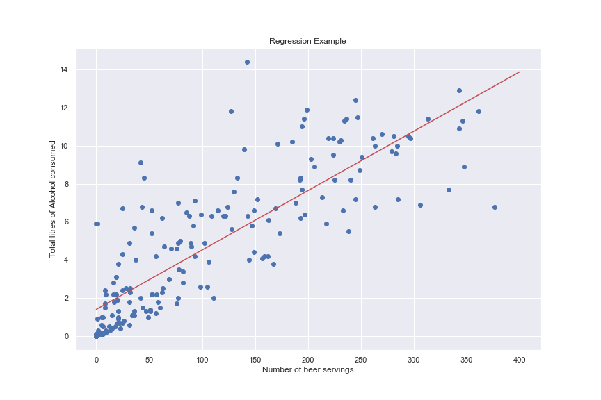
While linear regression can be used to model simple scenarios, as the data complexity increases it becomes less useful.
Polynomial Regression
As the name suggests, Polynomial regression is the approach where we model the data using higher degrees of the features. Linear regression is the case of Polynomial regression where all features are of degree 1.
For a dataset with data generating distribution \(P(X, Y)\), we need to find function \(\mathcal f\) that has the minimum generalization error.
For n degree polynomial regression, consider the hypothesis space \(\mathcal f \in \mathcal F\) of n degree polynomials with parameters \(\theta \in \mathbb R^{n}\). Then, the regression model can be written as:
\[\hat{\mathcal y} = \mathcal{f(x; \mathbf \theta)} = \sum_{d=0}^{n} \theta_{d}x^{d}\]For a degree 3 polynomial regression, we get
\[\hat{\mathcal y} = \theta_{3} x^{3} + \theta_{2} x^{2} + \theta_{1} x^{1} + \theta_{0}\]where, \(\theta_{0}=\epsilon\).
We will use the mean squared error loss to measure how wrong the predictions are. Our goal is to find the best value of \(\mathbf{\theta_{\star}}\) such that,
\[\begin{equation} \begin{aligned} \mathbf{\theta_{\star}} &= \mathop{argmin}_{\mathbf{\theta}} \mathcal{l}(y, f(x; \mathbf{\theta})) \\ &= \mathop{argmin}_{\mathbf{\theta}} \mathbb{E}_{\mathcal{(x, y)\sim}P(X, Y)} [(\mathcal{y - f(x; \mathbf{\theta})})^{2}] \end{aligned} \end{equation}\]We are basically taking the best approximation of parameter \(\theta\) that has the minimum empirical risk. This approximation can be used for further prediction.
We can also solve ordinary linear regression problems with the help of normal equations. Normal equations directly solve for linear regression providing us the optimal solutions directly. If \(X\) is our d-dimensional features matrix and \(y\) is our target, then the optimal parameter \(\theta_{\star}\) is;
\[\mathbf{\theta_{\star}^{d}} = (X^{T}X)^{-1} X^{T}y\]This equation directly gives the optimal solution without having to approximate our way with complex methods. So, why don’t we always use it?
It turns out that with increase in dimension of X and number of examples in the dataset, it can be computationally expensive to compute the inverse of the feature matrix. Since, we are required to find the inverse, this method is not useful in cases where the feature matrix is singular i.e. which has a zero determinant (Most libraries have a pseudo-inverse method to handle such cases, though).
Logistic Regression
Logistic regression is a linear model often used in classification problems, particularly binary classification in which we have two classes or categories to predict. Logistic regression predicts the probability of a certain class given the features.
\[P(Y = y \mid X = x)\]Can we use Linear regression for Classification?
Yes, but you probably shouldn’t. Linear regression is great for working with targets in the space of real numbers. In classification problems, where we often represent the classes numerically, linear regression might try to find relations between the classes while they could be completely independent. Consider, that we are trying to predict if the given image is a dog, cat or neither. The classes could be represented as 1, 2 and 3 for dog, cat and neither respectively. Linear regression might relate the classes with their numerical representation, thinking that they are continuous. Linear regression might be somewhat better in binary classification problems.
Logistic regression uses the sigmoid activation function to map the features to a continuous range from zero to one. The sigmoid function is defined as;
\[\sigma (x) = \frac{1}{1 + e^{-x}}\]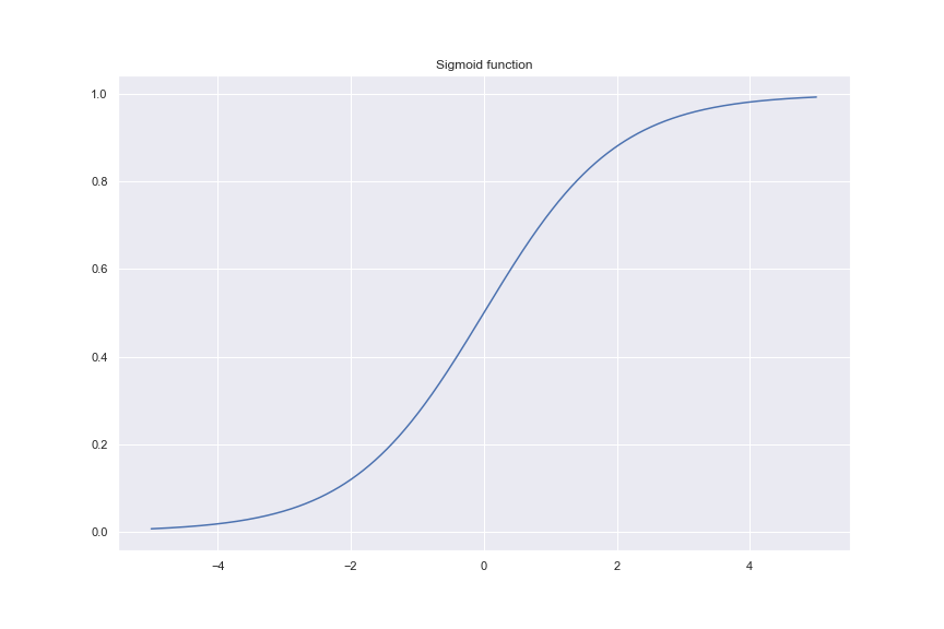
As \(x \to -\infty\) the sigmoid saturates to zero and as \(x \to \infty\) it saturates to 1. So, it is important that we scale our features to the range of (0, 1) for better convergence.
For general linear models like logistic regression, we have the model;
\[y = \theta_{1}x + \theta_{0}\]With the logistic function,
\[\sigma (y) = \frac{1}{1 + e^{-(\theta_{1}x + \theta_{0})}}\]where, \(\sigma (y) \in (0, 1)\).
If we define a threshold (say 0.5) for the output value, we can use it for classification as below.
\[c = \begin{cases} 1, & \text{if $\sigma$(y) $\ge$ 0.5} \\ 0, & \text{otherwise} \end{cases}\]Under-fitting and over-fitting
Consider that the hypothesis space \(\mathcal F\) we chose, has functions that are too simple (which fails to model the data accurately) or too complex (which might fit the data too much, thus losing generalization) with respect to the true data generating distribution. These are sub-optimal functions which fail to generalize the dataset decently.
Let function \(\mathcal f\) which maps from the input \(\mathcal X\) to the targets \(\mathcal Y\) be a function in our hypothesis space then, \(\mathcal{Y^{X}}\) is the set of all such functions, \(\mathcal{f: X \to Y}\).
The minimal error achievable by our model is known as the Bayes error or Bayes risk, \(R_{B}\). It is the minimal expected risk over all possible functions.
\[R_{B} = \mathop{min}_{\mathcal{f \in Y^{X}}} R(\mathcal{f})\]and the model that achieves this minimum is Bayes model, \(\mathcal f_{B}\). It is the theoritical limit to our model estimation.
The ability to learn from the data for a model is its capacity. In other words, the capacity of a learning algorithm is its ability to find a good model \(\mathcal{f \in F}\) for any function, regardless of its complexity. Often times, a more complex model has a higher capacity than simpler ones. For example, a neural network with multiple hidden layers can represent much complex functions than a linear regression model.
In practice, the capacity of a model can be controlled through hyper-parameters of the learning algorithm. For example,
- The degree of the family of polynomials (A higher degree polynomial can represent more complex functions)
- The number of layers in a neural network (capacity increases with the increase in number of layers)
- The number of training iterations (As we train more on the dataset, our model might fit more closely to the data)
- Regularization terms (Often used for decreasing the capacity of a model, deliberately to prevent over-fitting)
Under-fitting
If the capacity of \(\mathcal F\) of our model \(\mathcal f\) is too low, such that it cannot capture the patterns in the data, then \(\mathcal f_{B} \notin \mathcal F\) and the difference between the expected risk of any \(\mathcal f\) and the bayes risk, \(R_{B}\) i.e \(R(f) - R_{B}\) is very large for any function \(\mathcal{f \in F}\), including optimal model \(f_{\star}\) and estimated model, \(\mathcal f_{\star}^{\mathbf d}\). Such models \(\mathcal f\) are said to underfit the data.
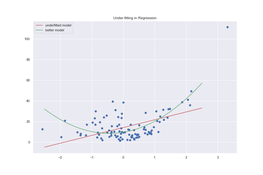
An underfitted model is said to have high bias and such models cannot fit the data to the required level, hence it leaves the model wanting. To better fit the data, we can use a more complex model, with higher capacity, that can fit the data well or we can reduce regularization, if any.
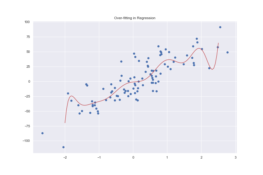
Over-fitting
If the inability of a model to fit data properly is a problem, then a model that fits the dataset so much that a single example is enough to sharply affect the decision parameters of a model is said to have overfitted to the dataset. If the capacity of \(\mathcal F\) is too high, then the bayes model, \(\mathcal f_{B} \in \mathcal F\) or \(R(f_{\star}) - R_{B}\) is very small. However, because of the high capacity of the hypothesis space, the empirical risk minimizer \(\mathcal f_{\star}^{d}\) could fit the data extremely well such that,
\[R(\mathcal f_{\star}^{d}) \ge R_{B} \ge \hat R(\mathcal f_{\star}^{d}, \mathbf d) \ge 0\]In this situation, the model fits too well to the data distribution but loses ability to generalize to newer examples. Thus, \(\mathcal f_{\star}^{d}\) is said to overfit the data and is said to have higher variance.
Our goal is to achieve a balance between the way the model fits to the dataset without affecting the generalization. we want to adjust the capacity of the hypothesis space such that the expected risk of the empirical risk minimizer gets as low as possible.
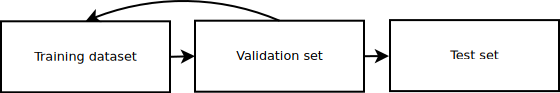
To evaluate a model, we often use a validation set (a small portion of the dataset dedicated for hyper-parameter tuning) to observe the model performance during training. But, as we train a variety of models over the same training and validation set over multiple runs, it is possible that the model might infer data from the validation set and start fitting to it. In such a case, the validation set is not an accurate measure of our model performance. Thus, we often have a separate test dataset (untouched during training) to test the model performance after we have a decent model performance on the validation set. It is very important that the test set not be tampered with during the training.
Bias-variance decomposition
Let us consider a single example, \(x\) and the prediction of the empirical risk minimizer given \(\mathcal x\) as \(\hat{Y} = \mathcal f_{\star}^{d}(\mathcal x)\). Then, the local expected risk of \(\mathcal f_{\star}^{d}\) is;
\[\begin{equation} \begin{aligned} R(\mathcal f_{\star}^{d}\mid \mathcal x) &= \mathbb E_{y \sim P(Y|x)} [(\mathcal{y} - \mathcal{f}_{\star}^{d}(x))^2] \\ &= \mathbb E_{y \sim P(Y\mid x)} [(\mathcal y - \mathcal f_B(x) + \mathcal f_{B}(x) - \mathcal f_{\star}^{d}(x))] \\ &= \mathbb E_{y \sim P(Y\mid x)} [(\mathcal y - \mathcal f_{B}(x))^2] + \mathbb E_{y \sim P(Y\mid x)} [(\mathcal f_B(x) - f_{\star}^{x})^2] \\ &= R(\mathcal f_{B} \mid x) + (\mathcal f_B(x) - \mathcal f_{\star}^{d}(x))^2\\ \end{aligned} \end{equation}\]where,
- \(R(\mathcal f_B \mid x)\) is the local expected risk of the Bayes model and cannot be reduced.
- \((\mathcal f_B(x) - \mathcal f_{\star}^{d}(x))^2\) is the discrepancy between the bayes model, \(\mathcal f_B\) and the expected risk minimizer, \(\mathcal f_{\star}^{d}\).
Formally, the local expected risk reduces to:
\[\begin{equation} \begin{aligned} \mathbb E_d [R(\mathcal f_{\star}^{d} \mid x)] &= \mathbb E_d [R(\mathcal f_{B} \mid x) + (\mathcal f_B(x) - \mathcal f_{\star}^{d}(x))^2]\\ &= R(\mathcal f_B \mid x) + \mathbb E_d [(\mathcal f_B(x) - \mathcal f_{\star}^{d}(x))^2] \\ &= R(\mathcal f_B \mid x) + (\mathcal f_B(x) - \mathbb E_d [\mathcal f_{\star}^{d}(x)])^2 + \mathbb E_d [(\mathbb E_d [\mathcal f_{\star}^{d}(x)] - \mathcal f_{\star}^{d}(x))^2]\\ \end{aligned} \end{equation}\]This decomposition is known as the bias-variance decomposition.
- \(R(f_B \mid x)\) is the noise term and is the irreducible part of the expected risk.
- \((\mathcal f_B(x) - \mathbb E_d [\mathcal f_{\star}^{d}(x)])\), is the bias term and it measures the discrepancy between the average model and the Bayes model.
- \(\mathbb E_d [(\mathbb E_d [\mathcal f_{\star}^{d}(x)] - \mathcal f_{\star}^{d}(x))^2]\) is the variance term and it quantifies the variability of the predictors.
Bias-Variance Tradeoff
- A model with higher bias is underfitting to the data. If we do not select a model with enough capacity or we reduce the capacity of a model then \(f_{\star}^{d}\) will fit the data less on average which increases the bias term.
- A model with higher variance is overfitting to the data. If we select a model with high capacity or we increase the capacity of a model, then \(f_{\star}^{d}\)